Practical Data Science: Promotion Effectiveness and Promotion Planning—Part 3

6-Step Process | Step 2 — Prepare Modeling Dataset (1/2)

Photo by Aexander Sinn on Unsplash

Welcome back to a series of articles on promotion effectiveness measurement and promotion planning! In Part 2, I discussed Step 1 of the overall process: (1) build a data foundation. Today, I will continue to discuss the next step—Step 2: (2) prepare a modeling dataset.

In case you missed the previous articles, links to Part 1 and Part 2 of this series are shown below.

Practical Data Science: Promotion Effectiveness and Promotion Planning — Part 1 | by Minha Hwang | Towards Data Science

Practical Data Science: Promotion Effectiveness and Promotion Planning — Part 2 | by Minha Hwang | Nov, 2022 | Towards Data Science

Step 2: Prepare a Modeling Dataset

Foundational data collected in the central data repository for promotion effectiveness modeling are at a lower grain than the required modeling dataset. Thus, we need to properly aggregate the data at the level of modeling grain. This design: lower grain foundational datasets and a higher grain modeling dataset, is intentional for us to ensure flexibility in the choice of modeling grains and feature engineering in the modeling dataset preparation stage. It is always possible to aggregate the data, but we can’t disaggregate data once aggregation is conducted.

In addition to aggregation, we need to create new data columns (i.e., new features), which align with modeling specifications. Therefore, aggregation, filtering, and feature engineering are required to go from foundational data to the modeling dataset. This step involves (1) data quality checks such as outlier analyses and summary statistics, and visual inspection, (2) (store) clustering analyses if promotion zones or pricing zones were not defined before, (3) data filtering and aggregation, (4) feature engineering to create derived columns, and (5) post modeling dataset checks to ensure data aggregation and feature engineering are conducted properly: e.g., data join checks, summary statistics checks, and time trend checks. Before describing these in detail, I have summarized the design consideration for the modeling dataset

1. Modeling grain (proper aggregation)

There are 3 primary dimensions that define the aggregation level of modeling grain. I have described recommended choices below.

(1) Time — Day vs. Week: Weekly data are a very common choice in the industry, but I would recommend daily data. Weekly data would work fine and help with the modeling of low-sales velocity products. However, this can create “aggregation bias”, if you are not careful. This is more common for multi-market retailers or national manufacturers. Multi-market retailers (e.g., Kroger) typically grew with M&A and local chain banners tend to stick with different promotion calendars. When promotion calendar weeks (e.g., Wednesday to Tuesday) of certain local market chains are misaligned with a common database week (e.g., Sunday to Saturday), using the weekly POS data leads to biased estimates of promotion ROI and price elasticities (usually underestimated). This is visually demonstrated in Figure 1 by comparing typical IRI or AC Nielsen data with the split week problem with the ground-truth data (aggregated from another daily dataset with a proper promotion week definition.)

We call this data aggregation bias problem a “split week” problem since the real promotion week data are artificially split into two database weeks. Figure 1 above shows actual sanitized data in the cereal product category at Ralphs chain in Southern California. We compare IRI unit sales and price data (i.e., misaligned data) with promotion week aligned data (which is a proxy of properly aggregated data from Kroger: 84.51: We have created proxies for both by using household panel data for this example since Kroger 84.51 data are not accessible for research. However, this is based on multiple consulting project experiences.) With the blending of promotion week data with non-promotion week data, promotion peak volume is understated in IRI data. In contrast, off-promotion sales (a week following the promotion week) are overstated in IRI data. Net prices are overstated during the promotion week and understated in non-promotion week in IRI data. These patterns usually lead to underestimation of promotion ROI and downward biases in price elasticities. Even more, the net prices from IRI or AC Nielsen data do not correspond well to actual regular prices or promotion prices in the accounts with a “split week” problem, as shown in Figure 1.

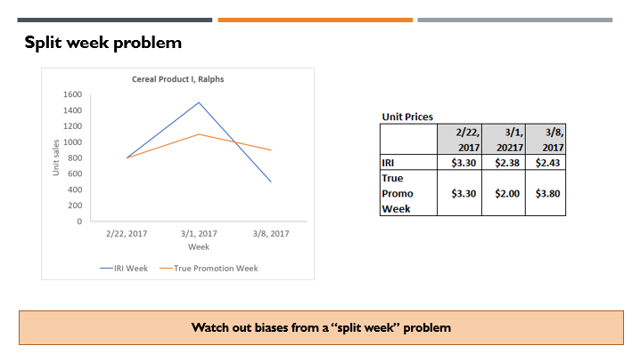
Figure 1: Image by Minha Hwang

Moreover, daily deals become more common recently, which results in a partial-week promotion. Daily data week will be more robust against aggregation biases from daily deals. If you work with a retailer or a manufacturer with a single promotion week definition without daily deals, weekly data would be appropriate as time grain.

(2) Product —Brand, UPC, vs. Brand-Pack: Most of the academic research on promotion modeling used brands as a level of analysis (Commercial Use of UPC Scanner Data: Industry and Academic Perspectives, Marketing Science, 1999). This is partly due to the fact that computing power was limited when promotion modeling was popular in Marketing Science in early 2000. However, the real product that you have to manage, and measure is at the UPC level. Thus, UPC is a more natural choice as a grain for the product. Moreover, you can find that price elasticities do change by different package sizes (e.g., 2L bottle vs. 12-ounce 12-pack cans) and flavors (e.g., Regular vs. Diet) within the same brand. For certain product categories, product line pricing is common, in which all UPCs within the same product line have the same regular prices and promotion prices. As long as prices and non-price marketing supports are common, it is fine to aggregate UPCs to a higher level. As an example, for a soft drink category, regular prices and promotional prices are maintained the same for all UPCs with different flavors (Coca-Cola Diet, Coca-Cola Regular) when the package size is the same. Brand/pack size aggregation can be proper in this case.

(3) Location — Store vs. Zone: The simplest choice here would be to use “store” as a grain since a single store should have the same promotion. This also gives you the flexibility to tailor promotions or pricing at the store level. On the flip side, the unit sales of the product at the store level are quite noisy (especially for tail UPCs with frequent zero sales per day or per week). Thus, in most cases, it is preferred to aggregate store-level data to higher geographical units as long as the promotion is homogeneous within the geographical units. Again, if you are not careful and aggregate stores with different promotion schedules, aggregation bias can result, which will distort promotion ROI measurements and price elasticity estimates (Using Market-level Data to Understand Promotion Effects in a Non-linear Model, Journal of Marketing Research, 1997) Most of the multi-market retailers assign promotion zones (and price zones) to stores. Within the same promotion zones, promotion prices are the same. Similarly, within the same price zones, regular prices are the same. Pricing departments (in charge of regular prices) are commonly separate from promotion departments (in charge of promotion prices), thus it is possible to observe differences in pricing zones and promotion zones. Ideally, a common zone both for regular prices/promotional prices are preferred, but you can differences from time to time. Thus, you can either use (1) promotion zone as modeling grain (if pricing/promotion zones are the same), or (2) pricing/promotion zone combination as modeling grain (if pricing zones are different from promotion zones.) This will ensure that you can avoid “aggregation” biases and make data more robust since random noises at store/product level will cancel out with the higher-level aggregation. After data aggregation is done, it is important to compare overall summary statistics (e.g., # of unique days, # of unique products, total revenue, total unit sales) before and after aggregation to ensure that there are no significant data loss or SQL coding errors. It also helps to plot time series to make sure that there are no irregular anomalies in the data. I will make this more concrete with actual POS data and code examples in the next article.

2. Filtering of data

For business datasets such as POS data, it is quite common to have outliers. Thus, outlier detection (based on typical anomaly detection algorithms with pre-specified thresholds) needs to be carried out to filter out outliers, which are most likely to be based on incorrect data entries. Some UPCs are failed products with almost no real sales. These UPCs add noise and are practically irrelevant to the business. Thus, it is common to apply unit sales thresholds to filter out UPCs with very low levels of sales. There can be only 1 or 2 inventories of certain UPCs from the previous season, which again is practically irrelevant. You can filter these UPCs out as well by checking # of weeks with unit sales. After filtering with several criteria, you can check what % of revenue or (equivalent) unit sales are maintained to ensure that you are not filtering data too much. Usually, 95% — 99% of revenue will be maintained after proper data filtering. In the next article, I will demonstrate filtering with actual POS data and Python code samples.

3. Feature engineering (derived columns)

In addition to aggregation and filtering, a major task in modeling dataset generation is creating derived feature columns, which are mapped to the causal demand model specification. Shown below are typical columns that you need to create for the simplest model as a toy example.

(1) Primary keys: UPC, Day, Promotion Zone ID

(2) Volume (in equivalent units): Unit sales x volume equivalent

(3) Own price: Unit price for the focal UPC

(4) Promotion tactics: Initially categorical variables (Must Buy 2, Buy 1 Get 1 Free, % Discount, Absolute Dollar Discount, etc.) This will be one hot-encoded to create separate dummy variables for each promotion tactic type.

(5) Non-price promotion: Feature indicator (0/1), Display level (High/Medium/Low), Coupon indicator (0/1). A binary indicator is the simplest. If more nuanced measurements are desired, you can separate the front page of features from the inside and back pages. Cases on the display (i.e., continuous variable) can be used instead of display levels. It is well known that a front-page feature on Sunday is more effective, especially with large product advertising sizes. However, this will cost more.

(6) Competing product prices: Ideally, you should figure out what sets of products are considered similar and put the prices of these products, which will change by focal UPC. However, this is difficult unless you have other datasets, which provide information for product similarity. Product similarity data can come from product switching data from loyalty cards for retailers, household panel datasets (e.g., Nielsen Homescan), Amazon search data, or text mining of product descriptions. Since own price elasticity (on average -2.5) is an order of magnitude large than cross-price elasticities (impact from the price changes of competing products, 0.1 ~ 0.3), it is fine to only control competing prices in an aggregate price index for initial promotion modeling journey. The aggregate competing price index can be computed by calculating (the revenue of products in the same subcategory) / (unit sales of products in the same subcategory) after excluding the focal product. Using constant weights is more robust, but this simple weighting works fine if you want to keep things simple. For an application at scale, a more rigorous way of computation sometimes can be intentionally avoided if the impact on the final results is small and computing costs are large (i.e., engineering decision.) However, this does require careful testing to ensure that potential loss of robustness is small and manageable.

(7) Weekly dummies: To properly control weekly seasonality, we can also include one-hot encoded weekly dummy variables. Specifying this at the category (or sub-category level) balances # of variables with modeling flexibility

(8) Weekday indicators: If you are using daily data, it is a good idea to include weekday indicators (e.g., Monday, Tuesday, and Sunday) to capture different shopping patterns across weekdays.

(9) Trend variable: It is fairly common to have underlying trends. The simplest thing you can do is to include the week number variable and its polynomials (e.g., week number, week number squared.) It is also possible to apply the LOESS procedure or Holt-Winters procedure (i.e., exponential smoothing) to decompose seasonality and trends after price control as pre-processing.

(10) Cost: To calculate promotion ROI, the cost of the product (i.e., wholesale prices for retailers, or COGS for manufacturers) and the cost of promotions should be included in the modeling dataset.

(11) Log transformation: The simplest work-horse model that works well in practice is a mixed effect log-log demand model. This model uses log(unit sales in volume equivalent) as the dependent variable and log(unit price) and price variables. Thus, you need to apply log transformation to price and unit sales variables.)

(12) (Optional) product attributes: If you have access to product attribute data (e.g., product stub file from IRI) with clear ideas on what product attributes matter, you can also include product attributes. This will allow you to make predictions for new products, which were never sold before as long as the new product can be expressed as a combination of existing product attributes. Including product attributes will also give you an idea of what product attributes are more popular vs. less popular.

4. What to watch out

(1) Check price variation: One of the common mistakes is equating the size of data records with the richness of the dataset. For price and promotion modeling, what matters more is whether you have good price variation over time (within the same UPC/store) for a large % of products. In the example in Figure 2, Walmart has a larger dataset, but the Best-buy dataset would be more useful due to frequent price variation. One useful summary statistic that you can calculate is the coefficient of variation of prices (i.e., relative standard deviation: mean / standard deviation X 100%). In one of the extreme examples, out of 15,000 products for dollar stores, only 300 products had a meaningful variation of prices to be useful for price modeling in one of my consulting projects.

Figure 2: Image by Minha Hwang

(2) Ensure enough history: Seasonality and trends are very common. To properly control them, you need to have at least 2–3 years of data. Covid caused a structural break, which makes the identification of seasonality harder with the recent data.

(3) Aggregation bias: In the discussion above on modeling grain, you may have noticed that the central theme is avoiding “aggregation” bias. It is okay to aggregate as long as promotion conditions are homogeneous. However, if you start to aggregate data with different promotion conditions, you are starting to induce biases (usually along the direction of under-estimating price elasticities.)

(4) Cross-section only: There can be a request to use only cross-sectional data (multiple geographic units/products with a single time period) to conduct causal promotion demand modeling. This will be very difficult, which requires special modeling techniques (e.g., spatial econometrics) and strong assumptions. Most useful (causal) price variations in the data are from within product/store across time variations. Without multiple price variations with enough histories, it is not possible to measure promotion ROI or price elasticities properly.

(5) Dependency with modeling choice: There is a very strong dependency between model specification and modeling dataset creation. Therefore, it is very important to be clear about what model specifications you will try and be more inclusive about potential feature columns to create. Without proper planning, you may have to go back to modeling dataset creation and redo the work. This can be even more painful if you have to do data fusion and combine datasets with different levels of data (e.g. product similarity from loyalty card data + store-level POS data.)

In the next article, I will make these ideas more concrete by utilizing public POS data (Dominick’s dataset, Kilts Center of Marketing, University of Chicago) and SQL / Python code samples.

Note

Promotion modeling was considered a largely solved problem in academia around 1999. Academic research on promotion has been less active recently except for changing the causal demand modeling method from a log-log model to the aggregate discrete choice model. In contrast, large-scale adoption of promotion ROI measurement and promotion modeling as a solution only started around 2014 by major consulting firms in the United States. These models were implemented before, but those were limited in scope: only by a handful of retailers or manufacturers (e.g., CVS, Proctor & Gamble.) This is a very common pattern for the adoption of new methods from academia to the industry with computing power increase and more data education (lagged by 10–20 years.) The reality is that promotion modeling is far from a solved problem if you try to implement this on a large scale. The connection of causal ML demand modeling with promotion optimization is not studied extensively both in academia and practice.

Reference

1. 8451: First-party retail data platform provided by Kroger. Includes store-level POS dataset and aggregate summary from loyalty cards, https://www.8451.com/
2. Randolph E. Bucklin and Sunil Gupta, Commercial Use of UPC Scanner Data: Industry and Academic Perspectives, Marketing Science, 1999
3. Markus Christen, Sachin Gupta, John C. Porter, Richard Staelin and Dick R. Wittink, Using Market-level Data to Understand Promotion Effects in a Non-linear Model, Journal of Marketing Research, 1997
4. Dominick’s Dataset, Kilts Marketing Center, University of Chicago

Practical Data Science: Promotion Effectiveness and Promotion Planning - Part 2

6 Step Process | Step 1 — Build Data Foundation

Photo by Nathalia Rosa on Unsplash

Welcome back to a series of articles on promotion effectiveness measurement and promotion planning! In my last post, I talked about business problems, key concepts, and the importance of this use case. Today, I will describe (1) a 6-step process to build a promotion effectiveness measurement and planning solution and (2) the Step 1 of the overall process: Building data foundation.

Promotion Planning Solution Building: 6 Steps

Figure 1: Image by Minha Hwang

The 6 steps of promotion planning solution building are as follows:

(1) Build data foundation

(2) Prepare modeling dataset

(3) Causal demand modeling: The main outputs from the causal demand model are price elasticity, promotion tactic lift, and non-price promotion lift

(4) Synthesize modeling insights

(5) Build a promotion simulator

(6) Promotion (re)planning

Key activities for each step are summarized above in Figure 1. I will describe details of each step in this series of articles. In this article (part 2), I will focus on “Build data foundation.”

Step 1: Build Data Foundation

This step is foundational and causes most mistakes and problems. Recently, the importance of data foundation is being recognized and emphasized more, as shown in the “data-centric AI” by Andrew. Ng. In terms of required efforts, this step takes 2-to-6-month efforts of 1 or 2 full-time data engineers, who are guided by more senior data architect (part-time) and data scientists who will work on causal demand modeling. Please note that you have to plan enough buffers, especially when this step was not done in the past. In most cases, a central data lake with all the required data for promotion effectiveness modeling is likely not be built yet, thus the data engineers and data scientists who are in charge need to reach out to multiple data owners in multiple internal departments and external syndicated data providers and data vendors (if available).

The data foundation tends to be a use-case specific. Thus, this is usually considered as business domain knowledge that will be picked up from on-the-job training. Thus, this is least taught in academic programs except for technical SQL training. Making it even worse, many companies do not maintain high quality data schema and data dictionaries for many internal databases. I have noticed that many junior data scientists and data engineers struggle most with this step since a clear guideline and practical tips are rarely provided.

Raw data tend to be company and situation specific. Thus, there is no cookie-cutter solution that you can apply. That said, once you clearly understand what data are essential vs. nice-to-have, you can avoid being overwhelmed by the number of databases, tables, and columns that you need to go through. I will cover 2 most common cases: (1) retailers (e.g., supermarkets such as Albertsons, Safeway, Kroger, department stores such as Macy’s, drug store such as CVS and Walgreens, convenience stores such as 7 Eleven), and (2) manufacturers (e.g., Kellogg and Proctor & Gamble). For the case of manufacturers, I will focus more on industry sectors where syndicated data providers such as IRI and Nielsen are available: i.e., frequently purchased consumer packaged goods (i.e., CPG companies.) Please note that data foundation in the central data lake are usually maintained at the lower aggregation level (e.g., stores instead of promotion zones) than the final modeling grain level.

Build Data Foundation: Retailer Case

(1) Central promotion effectiveness data repository

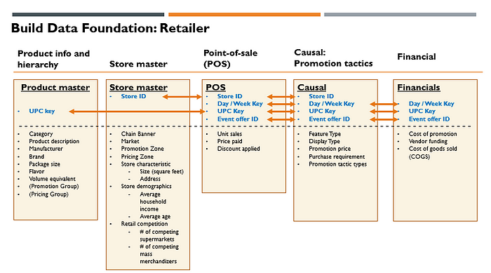
Figure 2: Image by Minha Hwang

Figure 2 shows the ERD (entity relationship diagram) of the central data repository that you need to build to have a 360-degree view on promotion effectiveness. Building this central data foundation is considered as a big win, since the required datasets are usually scattered across multiple departments and IT systems. Before I discuss each data domain in details, let me provide a few tips first.

1–1. Primary keys: For an effective central data repository, it is important to understand what primary keys are and which will be used to join data across tables. In this case, there are 4 primary keys: UPC key (i.e., product key based on UPC code, store ID (i.e., unique key for each store), day or week key (i.e., unique number for each week or day), and event offer ID (i.e., unique ID for each promotion event). One way to think about this is to imagine a 3-dimensional data cube (product | store | time), with additional key to attach promotion events and related information to this 3-dimensional data cubes. Please note that I have highlighted primary keys in blue in the ERD shown in Figure 2.

1–2. Aggregation level and aggregation bias: For a central data repository, it is recommended to keep data aggregation level as low as possible. It is always possible to aggregate at the later stage (e.g., feature engineering for modeling dataset). However, if you already aggregate the data to too high level, it is not possible to disaggregate later. Moreover, improper aggregation of dataset can cause biases in causal effect estimation. One well-known example of “aggregation bias” is when you aggregate data across stores with heterogeneous promotion activities. Another less-known example is “split week” bias, when you apply a common week definition to aggregate daily data to weeks. Because promotion calendars can have different promotion week definition across local markets (e.g., Sun — Sat vs. Fri—Thu), this will result data from non-promotion week and promotion week are blended in a common week definition for certain markets. If week is commonly defined as Sun — Sat for entire data and there are a few local markets which follow Fri—Thu promotion calendar, this blending will happen for all the stores in the local markets which follow Fri — Thu promotion calendar. It is a bit surprising that this happens quite frequently in practice (and even in the case of data from syndicated data providers.) I will give more details on this later in the modeling stage.

1–3. Data duration: At least 2–3 years of data are required to properly reflect seasonality and trends. Covid lock downs in Year 2020 and 2021 distorted normal seasonality and trends, thus extra care will be needed to handle data from these periods.

1–4. Executed vs. Planned: Oftentimes, there can be internal promotion planning database, which have promotion plans. One can be tempted to use this database as a source of “causal” table. However, it is very common to change plans at the last minute. Because of this, executed promotion prices and tactics can be very different from the original plans. Thus, it is highly recommended to use “executed” promotion prices and tactics instead of “planned” promotion prices and tactics.

1–5. Promotion with multiple price points: Beyond simple promotions with a single price point (e.g., 10% discount), there are complex promotions with multiple price points with certain requirements (usually in the form of multiple purchase requirements to qualify for quantity discounts.) With the complex promotion with purchase requirements, consumers can choose to either (1) buy a small quantity and pay regular prices or (2) buy large quantities and pay promotional prices. In the example shown below in Figure 3, if consumers decide to buy more than (or equal to) 4, they only need to pay $3.00 per each. However, if consumers decide to buy less than 4, they either need to pay the regular price of $4.99 per each (if they do not have a loyalty card) or pay the fallback promo price of $3.49 per each (if they have a loyalty card.) You can see that there are 3 possible price points in this example. The net price aggregated at store level for a given week for this product would be weighted average from these 3 price points.

Figure 3: Image by Minha Hwang

1–6. Basket-wide or category-level promotion: There are basket-wide or category-wide promotion events, which make it hard to calculate discount amounts per item level. You may have to decide on certain promotion discount allocation rules in these cases. As an example, Safeway could have run “Mix & Match” promotion in the wine category, which gives additional 10% discount if you buy more than 6 bottles. In this case, in addition to the product-level promotion discounts, there were additional 10% discounts that consumers enjoyed if they decided to buy more than 6 bottles.

1–7. Personalized promotion: In the past coupons were usually distributed equally to all consumers in the past by distributing them to the mailboxes of consumers. However, personalized and more targeted coupon promotions are adopted by more sophisticated retailers. The key feature of this promotion is that only a subset of consumers is offered with the promotion discounts. Other consumers who did not receive personalized coupons still pay regular prices or product-specific discount prices before the personalized coupon promotion. The existence of multiple effective prices across consumers makes it more complicated for us to decide on what effective promotion prices (at aggregate level such as stores or promotion zones) we should use for promotion effectiveness modeling in these cases.

(2) Key Tool: Source to Target Mapping

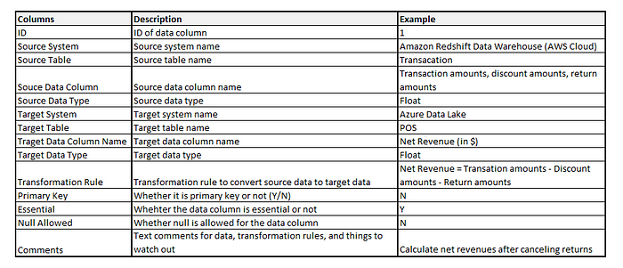
Data engineers and data scientists who work on this step have to go through multiple IT systems and discuss with multiple stakeholders. It is very easy to lose track of all the relevant facts, discussions, nuances, and watch outs. A tool, called as “Source to Target Mapping” can help greatly to keep track of key information and bring transparency on overall progress in this messy phase. This can be done, even as an excel file with multiple tabs for key types of data. If you want to be more systematic, you can make online version for easy sharing and update. Figure 4 shows key columns that you need in this tool with revenue as a sample data column.

Figure 4: Image by Minha Hwang

This tool makes it easier for data engineers and data scientists to understand how source data system / table / data columns are mapped to target data system / table / data columns. In addition, specifying transformation rule bring clarity on how source data columns are used to calculate target data columns. You can either enter (1) mathematical formulas or (2) SQL codes. In addition, this tool helps to clarify (1) primary keys, (2) whether the target column can allow null as data, (3) data types, and (4) data lake systems. Often times, the source systems are legacy inhouse IT systems (or even multiple excel files from certain departments.) In contrast, target system is most likely data lakes, powered by cloud service providers.

(3) Details on Key Data Domain

In this section, I discuss key data domains shown in Figure 2 in details.

3–1. Product master: Product master table contains product details with UPC key as a primary key. You can include product attributes (e.g., manufacturer, brand, pack size, flavor) together with product hierarchies (category, sub-category, department, aisle.) Almost always, there will be promotion groups or pricing groups where a group of products will share the same pricing or promotion discounts. It is good to capture these mapping. Volume equivalent needs additional explanation. For example, cola categories can have 2 products with different number of cans: 12 package / 12 Fluid Ounce Cans vs. 24 package / 12 Fluid Ounce Cans. Counting each product as 1 unit is not comparable, thus we need “volume equivalent” to convert units of product with different package sizes to comparable units. If we define “12 Fluid Ounce” as 1 volume equivalent, 1 unit of 12 package / 12 Fluid Ounce Cans is expressed as 12 volume equivalents. Similarly, 1 unit of 24 package / 12 Fluid Ounce Cans is expressed as 24 volume equivalents. Instead of using raw units, we use “volume equivalent” to measure volume (or unit sales).

3–2. Store master: Store master table provides details on stores. The primary key for this table is “Store ID”. In addition to chain banner (e.g., Safeway, Vons) and (local) markets, you can include (1) store characteristics (e.g., size of store), (2) store demographics (e.g., average household income, average age), and (3) retail competition intensity (e.g., # of competing supermarkets.) Zone pricing and Zone promotions are quite common. Thus, it is helpful to include this mapping information.

3–3. Point-of-Sale (POS): This is the most critical table with actual unit sales data with retail prices and discounts. The primary keys are (1) Store ID, (2) Day / Week Key, (3) UPC Key, (4) Event offer ID. Event offer ID provides a mapping to promotion event / tactic details from “Causal” table. This table is usually made from POS transaction database.

3–4. Causal: Causal table provide details on price and non-price (e.g., feature, display) promotions, which are not available in POS transaction data. The primary keys are (1) Store ID, (2) Day / Week Key, (3) UPC Key, (4) Event offer ID. As an example, transaction database provides (gross) revenues before any discounts and total discount amounts. However, it is hard to know purchase requirements (e.g., 4 to qualify for Must Buy 4 promotion), promotion tactics (e.g., Buy 1 Get 1 Free, Must Buy 2), promotion prices ($2.49 per each), presence of end-of-aisle display or feature advertising, just based on transaction database.

3–5. Financial: Financial table contains financial data for products, which can change over time. The primary keys are (1) UPC key, (2) day / week key, (3) Event offer ID. This table provides critical cost information from Finance department, which helps to measure profits beyond revenues. Note that activity-based cost accounting is usually used to allocate certain cost elements to the product level. In the case of retailers, promotion can be supported by additional funding from manufacturers (i.e., vendor funding). Thus, it is important to capture vendor funding to calculate true cost of running promotion. Separating out COGS (cost of goods sold) from cost of promotion helps for us to see what the main drivers of costs are.

Build Data Foundation: Manufacturer Case

Figure 5: Image by Minha Hwang

For the case of manufacturers, key data domains are similar. There are a few critical differences, which I call out below:

(1) Syndicated data providers: In the consumer-packaged goods industry, IRI and Nielsen collect data from retailers in supermarket (e.g., Albertsons, Safeway, Kroger), pharmacy (e.g., Walgreens, CVS), mass merchandiser (e.g., Wal-Mart, Target), and warehouse club (e.g., Costco, Sam’s Club) channels through their retail partnership, process the data, and provide data to manufacturers after subscription fees. Usually, retail data are aggregated to the account level, which is defined by chain banner / market combinations (e.g., Kroger — Dallas.) Therefore, this will be the lowest level of data grain. Note that CPG manufacturers can have a view on their competitors since syndicated data providers provide data on competing manufacturers as well. In addition, at least for “featured” promotions, CPG manufacturers can collect promotion tactic details (e.g., Must Buy 4 at $2.99) from a service, called Numerator. Numerator scans feature advertising inserts and generate data tables for featured promotions. Syndicated data provides also offer product master, market demographics, and chain characteristics. This situation is very different in other industries (e.g., Consumer Electronics or High-Tech), where these kinds of service is not available. In those cases, manufacturers are half-blind, since they can track their own promotion data, but not competitor promotion data. The best external data for High-Tech or Consumer Electronics industries are provided by NPD as household panel data (instead of POS data from retailers.) In case the manufacturers are working as category captains for select chains, that could another good source of data for promotion effectiveness measurement.

(2) Sell-in vs. Sell-through: Manufacturers can be tempted to use shipment data to retailers (sell-in) instead of retail sales data (sell-through.) This is a bad idea due to forward buying from retailers. Retailers can stockpile their inventories when there are good deals, but this may not move from retailers to consumers. Thus, it is important to use retail sales data instead of factory/distribution center shipment data.

(3) Wholesale prices vs. retail prices: It is less common for manufacturers sell directly to consumers (i.e., DTC). Manufacturers first sell to retailers, and retailers sell to final consumers. There can be intermediate wholesalers / distributors in the picture as well. Because of this, the topline for manufacturers will be different from final retail prices. Retailers add additional retail margins on top of manufacturer margins (i.e., double marginalization). For manufacturers, having visibility for both manufacturer margins and retailer margins are important to have data-driven discussions with retailers. Thus, in the financials table, gross/net revenue per unit of manufacturers are included together with retailer profit. It is also important to track regular price reduction allowance (EDLP allowance), fixed trade cost, and variable trade cost.

Hope you find Step 1 of the process useful. In the next article (Part 3), I will focus on Step 2 and discuss how we can create modeling dataset from the central data repository that I described in Part 2.